Understanding Machine Learning Models: From Supervised to Unsupervised Learning

Introduction to Machine Learning

Machine Learning (ML) is a subfield of artificial intelligence that empowers computer systems to learn from data without being explicitly programmed. Instead of following predefined rules, ML algorithms build a mathematical model based on sample data, known as “training data,” in order to make predictions or decisions without being explicitly programmed to perform the task. This ability to learn and adapt from experience is what makes machine learning a transformative technology, driving innovation across diverse sectors from healthcare and finance to entertainment and autonomous vehicles.

At its core, machine learning is about identifying patterns and relationships within data. These patterns can then be used to make informed predictions or classifications on new, unseen data. The process typically involves feeding large datasets to an algorithm, allowing it to identify correlations, trends, and anomalies. The more data an algorithm is exposed to, the better it becomes at recognizing these patterns and making accurate inferences. This iterative process of learning from data, evaluating performance, and refining the model is central to the machine learning paradigm.

The rise of machine learning has been fueled by several factors: the exponential growth of data (Big Data), advancements in computational power (e.g., GPUs), and the development of sophisticated algorithms. These elements have converged to enable the creation of highly complex and accurate models that can tackle problems previously considered intractable for traditional programming approaches. Understanding the different types of machine learning and their underlying principles is crucial for anyone looking to leverage this powerful technology.

Types of Machine Learning: Supervised, Unsupervised, and Reinforcement Learning

Machine learning algorithms are broadly categorized into three main types, each with distinct approaches to learning from data and solving different kinds of problems.

Supervised Learning

Supervised learning is the most common type of machine learning. In this approach, the algorithm learns from a labeled dataset, meaning each data point in the training set has a corresponding “correct answer” or output. The goal of supervised learning is for the model to learn a mapping function from input variables (features) to an output variable (target) so that it can accurately predict the output for new, unseen inputs. The learning process is analogous to a student learning under the guidance of a teacher, where the teacher provides feedback (the correct labels) on the student’s answers.

Supervised learning problems are typically divided into two main categories:

• Classification: This involves predicting a categorical output. The model learns to assign input data points to one of several predefined classes. Examples include spam detection (spam or not spam), image recognition (cat or dog), and medical diagnosis (disease A, disease B, or healthy).
• Regression: This involves predicting a continuous numerical output. The model learns to predict a value within a range. Examples include predicting house prices, stock market trends, or temperature forecasts.

Common algorithms for supervised learning include Linear Regression, Logistic Regression, Decision Trees, Random Forests, Support Vector Machines (SVMs), and Neural Networks.

Unsupervised Learning

Unsupervised learning deals with unlabeled data, meaning the training data does not have any corresponding output labels. The algorithm’s task is to find hidden patterns, structures, or relationships within the data on its own. It’s like a student learning by observing and discovering patterns without any explicit guidance or correct answers. Unsupervised learning is particularly useful for exploratory data analysis, data compression, and identifying anomalies.

Key applications of unsupervised learning include:

• Clustering: This involves grouping similar data points together into clusters. The algorithm identifies natural groupings within the data based on their inherent similarities. Examples include customer segmentation (grouping customers with similar purchasing behaviors), document clustering (grouping similar articles), and anomaly detection (identifying unusual patterns that don’t fit into any cluster).
• Dimensionality Reduction: This technique aims to reduce the number of features or variables in a dataset while retaining as much important information as possible. This can help in visualizing high-dimensional data, reducing computational complexity, and mitigating the curse of dimensionality. Principal Component Analysis (PCA) is a popular dimensionality reduction technique.

Common algorithms for unsupervised learning include K-Means Clustering, Hierarchical Clustering, and Principal Component Analysis (PCA).

Reinforcement Learning

Reinforcement learning is a type of machine learning where an agent learns to make decisions by interacting with an environment. The agent receives rewards or penalties based on its actions, and its goal is to learn a policy that maximizes the cumulative reward over time. This trial-and-error approach is inspired by behavioral psychology and how humans and animals learn. There is no predefined dataset; instead, the agent learns through continuous interaction and feedback from its environment.

Examples of reinforcement learning applications include training autonomous vehicles, developing game-playing AI (e.g., AlphaGo), robotics, and optimizing resource management in data centers. The agent learns to perform a task by exploring different actions and observing their consequences, gradually refining its strategy to achieve its objective.

Key Steps in the Machine Learning Workflow

Regardless of the type of machine learning, most ML projects follow a general workflow. Understanding these steps is crucial for building effective and robust machine learning models.

1. Data Collection

The first and often most critical step is collecting relevant data. The quality and quantity of data directly impact the performance of the machine learning model. Data can come from various sources, including databases, APIs, web scraping, sensors, and more. It’s essential to ensure the data is representative of the problem you’re trying to solve and that it’s ethically sourced.

2. Data Preprocessing

Raw data is rarely in a format suitable for machine learning algorithms. Data preprocessing involves cleaning, transforming, and preparing the data. This step includes:

• Handling Missing Values: Deciding how to deal with incomplete data (e.g., imputation, removal).
• Feature Engineering: Creating new features from existing ones to improve model performance. This often requires domain expertise.
• Data Transformation: Scaling, normalization, or encoding categorical variables.
• Splitting Data: Dividing the dataset into training, validation, and test sets. The training set is used to train the model, the validation set to tune hyperparameters, and the test set to evaluate the final model’s performance on unseen data.

3. Model Selection

Choosing the right machine learning model depends on the problem type (classification, regression, clustering, etc.), the nature of the data, and the desired performance characteristics. There isn’t a one-size-fits-all model; often, several models are experimented with to find the best fit.

4. Model Training

In this step, the selected model is trained using the training data. The algorithm learns the patterns and relationships by adjusting its internal parameters to minimize the difference between its predictions and the actual outcomes (in supervised learning) or to discover inherent structures (in unsupervised learning).

5. Model Evaluation

After training, the model’s performance is evaluated using the test set (and validation set during development). Various metrics are used depending on the problem: accuracy, precision, recall, F1-score for classification; Mean Squared Error (MSE), R-squared for regression; silhouette score for clustering. This step helps in understanding how well the model generalizes to new data and identifies areas for improvement.

6. Model Deployment and Monitoring

Once a model is deemed satisfactory, it can be deployed into a production environment where it can make predictions on real-time data. However, the process doesn’t end there. Models need to be continuously monitored for performance degradation (model drift) and retrained periodically with new data to maintain their accuracy and relevance.

Example: Building a Simple Decision Tree Classifier in Python

Let’s create a simple example of a decision tree classifier using Python and the popular scikit-learn library. We’ll use a synthetic dataset for simplicity.

Prerequisites

Ensure you have scikit-learn and pandas installed:

pip install scikit-learn pandas

Code Example

Create a Python file named decision_tree_example.py:

import pandas as pd
from sklearn.tree import DecisionTreeClassifier, export_graphviz
from sklearn.model_selection import train_test_split
from sklearn.metrics import accuracy_score
from io import StringIO
from IPython.display import Image
import pydotplus

# 1. Create a synthetic dataset
data = {
    'Age': [25, 30, 35, 40, 45, 50, 28, 33, 38, 42, 48, 55],
    'Income': [50000, 60000, 75000, 80000, 90000, 100000, 55000, 70000, 85000, 95000, 110000, 120000],
    'Student': ['No', 'No', 'No', 'No', 'Yes', 'Yes', 'No', 'No', 'Yes', 'Yes', 'Yes', 'No'],
    'Buys_Computer': ['No', 'No', 'No', 'No', 'Yes', 'Yes', 'No', 'No', 'Yes', 'Yes', 'Yes', 'No']
}
df = pd.DataFrame(data)

# Convert categorical features to numerical using one-hot encoding
df_encoded = pd.get_dummies(df[['Age', 'Income', 'Student']], columns=['Student'], drop_first=True)
X = df_encoded
y = df['Buys_Computer']

# Split data into training and testing sets
X_train, X_test, y_train, y_test = train_test_split(X, y, test_size=0.3, random_state=42)

# 2. Initialize and train the Decision Tree Classifier
# max_depth is set to limit the tree size for better visualization
model = DecisionTreeClassifier(max_depth=3, random_state=42)
model.fit(X_train, y_train)

# 3. Make predictions on the test set
y_pred = model.predict(X_test)

# 4. Evaluate the model
accuracy = accuracy_score(y_test, y_pred)
print(f"Model Accuracy: {accuracy:.2f}")

# 5. Visualize the Decision Tree (requires graphviz and pydotplus)
# If you don't have graphviz installed, you can skip this part or install it:
# pip install pydotplus graphviz
# On Ubuntu: sudo apt-get install graphviz

dot_data = StringIO()
export_graphviz(model, out_file=dot_data, 
                filled=True, rounded=True,
                special_characters=True, feature_names=X.columns, class_names=['No', 'Yes'])

graph = pydotplus.graph_from_dot_data(dot_data.getvalue())
# Save the tree to a PNG file
graph.write_png('decision_tree.png')
print("Decision tree saved to decision_tree.png")

# Example prediction
new_data = pd.DataFrame([[32, 65000, 0]], columns=['Age', 'Income', 'Student_Yes'])
prediction = model.predict(new_data)
print(f"Prediction for new data (Age=32, Income=65000, Student=No): {prediction[0]}")

new_data_student = pd.DataFrame([[27, 58000, 1]], columns=['Age', 'Income', 'Student_Yes'])
prediction_student = model.predict(new_data_student)
print(f"Prediction for new data (Age=27, Income=58000, Student=Yes): {prediction_student[0]}")

Explanation

1. Synthetic Dataset: We create a small pandas DataFrame with Age, Income, Student, and Buys_Computer (our target variable). Student is a categorical variable, so we convert it to numerical using one-hot encoding.
2. Data Splitting: The dataset is split into training and testing sets to evaluate the model’s generalization ability.
3. Model Training: A DecisionTreeClassifier is initialized and trained on the training data. max_depth is set to 3 to keep the tree simple for visualization.
4. Prediction and Evaluation: The trained model makes predictions on the test set, and its accuracy is calculated.
5. Visualization: We use export_graphviz and pydotplus to generate a visual representation of the decision tree. This helps in understanding the decision rules learned by the model.
6. Example Prediction: We demonstrate how to use the trained model to make predictions on new, unseen data.

Running the Code

Save the file as decision_tree_example.py and run it from your terminal:

python decision_tree_example.py

**Expected Output (may vary slightly based on random_state and data):

Model Accuracy: 0.75
Decision tree saved to decision_tree.png
Prediction for new data (Age=32, Income=65000, Student=No): No
Prediction for new data (Age=27, Income=58000, Student=Yes): Yes

This example provides a hands-on understanding of how a decision tree model is built, trained, and used for making predictions.

Diagram: A Visual Representation of a Decision Tree

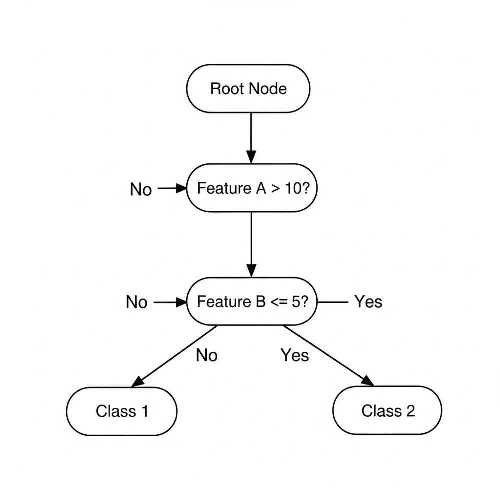
To further illustrate the structure and decision-making process of a decision tree, consider the following diagram:

This diagram depicts a simplified decision tree. It starts with a root node, which represents the initial decision point. Each internal node represents a test on an attribute (e.g., “Feature A > 10?”), and each branch represents the outcome of that test. The leaf nodes represent the final classification or decision (e.g., “Class 1”, “Class 2”). This visual representation helps in understanding how the model navigates through a series of decisions to arrive at a prediction.

Conclusion: The Evolving Landscape of Machine Learning

Machine learning has rapidly evolved from a niche academic discipline to a cornerstone of modern technology, fundamentally reshaping industries and daily life. The ability of algorithms to learn from data, identify complex patterns, and make intelligent predictions has unlocked unprecedented opportunities for automation, optimization, and discovery. From powering recommendation systems and fraud detection to enabling medical diagnoses and autonomous systems, ML models are at the forefront of innovation.

The distinction between supervised, unsupervised, and reinforcement learning provides a foundational framework for understanding the diverse applications of ML. Supervised learning, with its reliance on labeled data, excels in predictive tasks like classification and regression. Unsupervised learning, on the other hand, uncovers hidden structures in unlabeled data, proving invaluable for tasks such as clustering and dimensionality reduction. Reinforcement learning, through its trial-and-error approach, empowers agents to learn optimal behaviors in dynamic environments.

The machine learning workflow, encompassing data collection, preprocessing, model selection, training, evaluation, and deployment, highlights the iterative and data-centric nature of building ML solutions. Each step is crucial for developing robust, accurate, and deployable models. As the field continues to advance, we can expect even more sophisticated algorithms, more efficient training techniques, and broader accessibility to ML tools and platforms.

For aspiring practitioners, the journey into machine learning is both challenging and rewarding. A strong grasp of statistical concepts, programming skills (especially in Python), and an understanding of the underlying algorithms are essential. The proliferation of open-source libraries like scikit-learn, TensorFlow, and PyTorch has democratized access to powerful ML tools, enabling individuals and organizations to experiment and build their own intelligent systems. As data continues to grow and computational power becomes more accessible, machine learning will undoubtedly continue to drive the next wave of technological transformation, making it an exciting and impactful field to be a part of.